Machine learning models follow garbage in, garbage out policy: the quality of the model’s output is determined by what you feed to it. The final objective of most of the ML models is to find out the underlying data generating distribution and the performance of your model depends on a lot of parameters other than the model architecture. Why emphasize on it? Because this is what this post revolves around. I did this project with one of my friends, Serkan. We picked a standard model architecture (Unet) for semantic segmentation and a standard dataset (Cityscapes) and just by changing the data feeding strategy, and the loss function, we got pretty good mean IoU (Intersection over union) over different classes on the holdout set.
Semantic segmentation or dense prediction is a task where the objective is to label each pixel of an image with a corresponding class of what is being represented. I think of any supervised classification algorithm as trying to learn a partition in the input feature space such that if I sample a continuous region on any side of this partition, all instances in that region belong to the same class.
Coming to the Cityscapes dataset, there are around 2900 images in the training set and 500 images in the validation set. Training a CNN model on just 2900 images is probably not a good idea. For training a deep CNN, all classes should have sufficient representation in the training set and there should be enough images present in the dataset to prevent potential overfit. There are 20 classes in the Cityscapes dataset, out of which 19 classes point to a unique object and everything not belonging to these 19 labels belongs to the unlabeled class.
The first thing to target here is clearly the scarcity of images. For this, we augmented the data using random crops of 60% and 75% over the images. We trained the model in three phases, the first phase being where we show the 60% crops to the model, the second phase with 75% crops and in the last phase, the model gets to see the whole image. My understanding behind this is that this strategy allows the model to see less number of classes per image and learn them efficiently before moving forward.
After deciding the data augmentation strategy, the next decision to make was the loss function on which the model will be trained. For classification (and segmentation by extension), cross entropy is the to go loss function. We trained Unet with the above-mentioned training phases and Adam optimizer for three days until the errors stabilized and found the mean IoU over all classes to be 0.78 (0.836 being the benchmark on this dataset). Evaluating the cases where the model produces crappy output usually indicates the modifications needed to improve the model. On examining the outputs, we found that the model just puts everything in blobs i.e. it is really bad at learning the boundaries of the objects. You can see the output below:
Target segmentation map:
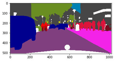
Predicted:
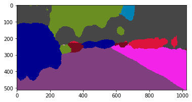
The way we combated this was by weighing the loss of the pixels on boundaries of objects more relative to the pixels within the objects. Thus, for each image, we create a mask which has value k (the weighing factor) for the pixels on the boundary and 1 for the pixels within the objects. All the class labels have general structures that the model can learn, except the background class which covers everything else. This imposes a challenge when generalizing the information that is learned for this class. It is expected that the model will make random predictions when there is a patch of the image that doesn’t fit well to any of the class definitions it had learned so far. For this reason, we associated prediction uncertainty with the background class. We quantify the prediction uncertainties by using dropouts. We used 3 different dropouts for the penultimate layer and then imposed a loss based on the variance between the predictions made by using these 3 outputs. Other than that, we multiply this variance with 1-prob(belonging to the background class) which enforces the model to predict the random patch as belonging to the unlabelled class whenever it is uncertain.
The final loss function thus becomes:
objective = mask * cross entropy loss + C * uncertainity loss * (1-prob(belonging to background))
Here, C is the factor determining how much importance to give to uncertainty loss relative to the cross-entropy loss. We trained the model using this objective function and this increased the validation set IoU to 0.8354. IMHO, the decisions regarding loss function, evaluation metrics, optimization procedure, etc are all which one should spend a substantial amount of time on before perturbing the architecture of the model. Some outputs spit out by the final model (actual image, prediction and target being the columns respectively):
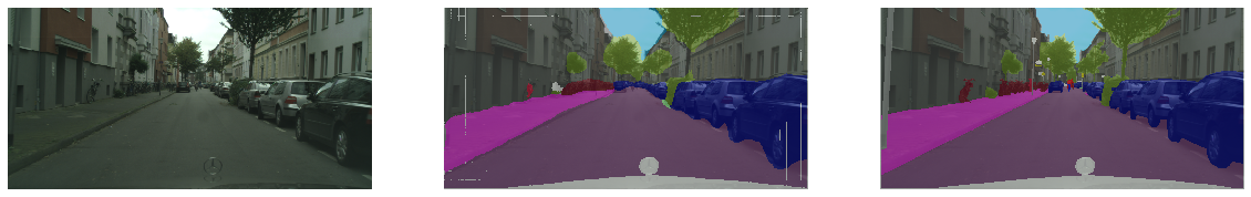
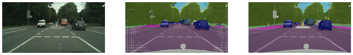
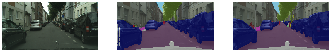
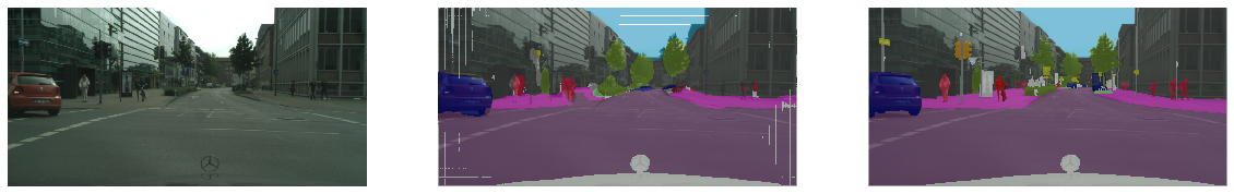
You can notice the streaks of white lines near the edges of the predicted segmentation maps. We are still trying to improve that. If you have any idea on how to correct that, let me know!
Show me the code
Code: GitHub
Thanks,
Ashwin